Structure-Preserving Difference Search for XML Documents
Erich Schubert
University of Berkeley, California
School of Information Management & Systems
erich@vitavonni.de
http://www.vitavonni.de/
Sebastian Schaffert
University of Munich
Institute for Informatics
Sebastian.Schaffert@ifi.lmu.de
http://www.wastl.net
François Bry
University of Munich, Germany
Institute for Informatics
Francois.Bry@ifi.lmu.de
http://www.pms.ifi.lmu.de/mitarbeiter/bry/
Keywords: Web; XML; Difference
Abstract
Current XML differencing applications usually try to find a minimal sequence of
edit operations that transform one XML document to another XML document (the
so-called "edit script"). In our conviction, this approach often produces
increments that are unintuitive for human readers and do not reflect the actual
changes. We therefore propose in this article a different approach trying to
maximise the retained structure instead of minimising the edit sequence. Structure
is thereby not limited to the usual tree structure of XML - any kind of structural
relations can be considered (like parent-child, ancestor-descendant, sibling,
document order). In our opinion, this approach is very flexible and able to adapt
to the user's requirements. It produces more readable results while still retaining
a reasonably small edit sequence.
|
1 Introduction
XML, the Extensible Markup Language, is nowadays used in a wide area of
applications, ranging from text oriented documents over languages aimed
at exchanging messages between peers to data centric formats for
exchanging and storing data. An important functionality is so-called
difference search (or "change
tracking") between documents. The output of a difference search has many
different applications, e.g. in revision control systems, in
bandwidth-saving "patch" systems that distribute only increments between
different versions of a document, and last but not least as a tool for
authors that allows for easily identifying the changes between different
versions of a document. Thus, the output of difference search systems
must both be processable by machines (e.g. to automatically merge changes of
documents) and be readable by human users.
While there exist several rather efficient approaches for machine processing, we
believe that none of them is particularly well suited for the last aspect, because all
existing approaches disregard the "human aspect". This "human aspect", however, is
particularly challenging, because it requires changes to be easily reproducible and
intuitive. Imagine, for instance, a collaboration system where several authors work on
the same XML document in parallel. In such situations, it is almost inevitable to
manually merge the changes from different authors. Representing the changes as the
"shortest edit-sequence", i.e. the shortest number of edit operations, usually does not
correspond to the changes that were actually performed by the changing author. Figure
1 illustrates this on two sample XML documents using the
Logilab XMLDiff system. While the Logilab XMLDiff result might be efficient for machine
processing, it does not reflect the actual changes in the document. Indeed, the
shortest edit-sequence would always be to completely remove the old document structure
and replace it with the new document structure.
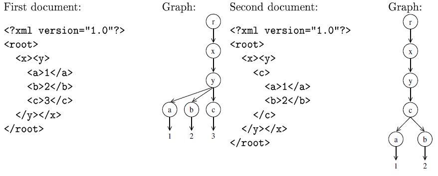
Figure 1:
Two sample XML documents; in the second document, the "a" and "b" elements have
been moved inside the "c" element, replacing the text "3" within it. The changes
produced by Logilab XMLDiff instead create a new root element, rename the old root
element to "x", rename the old "x" element to "y", rename the old "y" element to "c",
and finally remove the old "c" element.
[Graphic entity xmldiff-graphs — PMS-FB-2005-11/ExML05/EML2005SCHA031801.png]
|
We therefore propose a novel, very flexible, approach to XML difference search called
"structure-based differencing" that aims at addressing also this "human aspect", while
still retaining small and efficient "answers". Like other systems, our approach is
based upon the graph structure induced by an XML document, where the nodes represent
elements, and the edges represent relationships between elements. Instead of
minimising the edit sequence between the two structures for a fixed set of edit
operations, we then try to identify a maximum number of substructures of the graph
induced by the original document as substructures in the graph induced by the changed
document. Relationships occurring in such substructures are said to be retained. In a sense, one can say that in our approach we try
to find corresponding substructures, whereas most
other approaches try to find changes. This idea is
inspired by the Simulation Unification Algorithm we
presented in [Bry and Schaffert, 2002] and [Schaffert, 2004].
Note that we do not address the actual representation of deltas. For this purpose,
various representation formats are suitable, e.g. XUpdate [XUpdate]. Also, a visual representation (as in Emacs ediff) is
conceivable.
A salient aspect of our approach is that, in contrast to other structure-based
approaches, we consider not only the usual parent-child relationships but arbitrary
relations between nodes. This may include parent-child, but also sibling-sibling,
ancestor-descendant, or some user-defined relations. Furthermore, different kinds of
relationships can be assigned different levels of importance ("weights"), allowing a
very fine-grained control over the retained structure. In practice, trying to retain
parent-child as well as sibling relationships proved to be sensible choices for
differencing.
Besides these properties, the openness of our approach allows to add extensions
easily. For example, a "fuzzy matching" measure has been implemented in [Schubert, 2005].
This article is structured as follows: we first give a brief survey over other existing
approaches to XML difference search in Section 2 and show
their deficiencies. In Section 3, we introduce our
notion of document graphs, a data model extending
the usual tree model of XML data. Section 4
defines the notions of nodeset correspondence and retained relations. Section proposes a search strategy to find a nodeset correspondence with
maximal amount of retained relations. For this purpose, we suggest three different cost
functions that take into account various properties of the relations. We conclude with
perspectives for improvement.
2 XML Difference Search: State of the Art
Systems for difference search in XML documents can be roughly divided into two groups:
systems that operate on generic text content (and can thus also be used for XML
documents) and systems specifically designed for XML content. While not strictly
designed for XML difference search, we include the first group because it is still the
most widespread method of comparing XML documents. As a representative, we have chosen
the GNU Diffutils commonly found on different flavours of Unix and Linux.
2.1 Text-Based Difference Search: GNU Diffutils
The GNU Diffutils [GNU Diffutils] are a collection of tools used for
comparing arbitrary text documents, like plain text, program source code, etc. It
consists mainly of the two programs "diff" and "patch", where "diff" performs the
difference search and "patch" allows to apply deltas created by "diff" to an older
revision of a document. The GNU Diffutils are available on a wide range of platforms,
and are installed by default on most Unix and Linux systems. The Diffutils are
included here because they are fast, reliable, and still the most widespread system
for comparing XML documents. Other flavours of the GNU Diffutils using the same
comparison strategies can e.g. be found in Emacs ediff, the CVS and SVN versioning
systems, etc.
The "diff" application compares two documents line-by-line using an efficient
"longest common subsequence" algorithm (LCS) and marks all those lines that either
differ in the two documents or do not appear at all in one of the documents. The
output is both machine processable (e.g. by means of the "patch" util) and
conveniently readable by users, as it simply consists of removed lines (marked with
"-") and added lines (marked with "+"). Blocks of lines that have been moved to a
different location but are not part of the longest common subsequence found will
appear twice: removed at their old location and inserted at their new
location. Figures 2 and 3
illustrates the output of "diff" on two small sample XML documents.
Figure 2: GNU Diff: Two Sample XML Documents
<?xml version="1.0"?>        <?xml version="1.0"?>
<a>                          <a>
  <b>                          <b>
    <c/>                         <c/>
  </b>                           <c/>
  <b>                          </b>
    <c/>                     </a>
  </b>
</a>
|
Figure 3: GNU Diff: Output generated by "diff"; hand-made desirable output
The left column shows the output generated by GNU "diff" when comparing the
two sample documents of Figure 2. It is easy to see
that this delta does not reflect tree operations; a more intuitive, hand-crafted
delta is given in the right column.
  <?xml version="1.0"?>        <?xml version="1.0"?>
  <a>                          <a>
   <b>                          <b>
     <c/>                         <c/>
-  </b>                      +    <c/>
-  <b>                          </b>
     <c/>                    -  <b>
   </b>                      -    <c/>
 </a>                        -  </b>
                               </a>
|
The longest common subsequence algorithm used in GNU diff is fairly
straightforward. In its general form, it uses the three edit operations deleteChar,
insertChar, and updateChar, and tries to find a minimal sequence of operations that
transform the first document (of length n) into the second document (of length m). To
obtain a solution, it constructs a n × m matrix representing in each (i,j) cell
the necessary operations and associated costs to transform the prefix of length i
into the prefix of length j. Candidates are all paths in the matrix that end in the
cell (n,m). From those, the path with minimal cost is chosen. In this case, the
sequence of unmodified characters is the "longest common subsequence". Note that GNU
diff actually operates on lines instead of characters, but the principle is the same.
Being not designed specifically for XML data, GNU "diff" has three major deficiencies
when comparing XML documents:
- whitespace is significant, especially line breaks; two XML documents
representing the same data might not be recognised as equal by GNU diff
- line-based operations are not aware of the structure of XML documents and
do not correspond to tree operations; often, this may lead to a "mismatch" of
opening and closing tags in the delta (cf. Figure 3)
- ordering of elements may be irrelevant in an XML document (as can e.g. be
expressed by RelaxNG); GNU "diff" will consider reorderings as deletions and
re-insertions at a different position
On the other hand, GNU "diff" has also its benefits, which explain why it is still in
such widespread use:
- the algorithm is very efficient and fast
- it is available on almost any Unix machine, and included in dozens of
applications on all platforms
- the output is very easy to read and review
2.2 XML-Aware Difference Search
XML-aware difference search systems, like XyDiff [Cobéna et. al., 2002a],
LaDiff [Chawathe et. al., 1996], DeltaXML [La Fontaine, 2002],
X-Diff [Wang et. al., 2003], MMDiff [Chawathe, 1999], Logilab
XMLDiff [XMLDiff], and IBM's XML Diff and Merge Tools
[IBM XML Diff and Merge], operate on the tree structure defined by the
elements in XML documents instead of the pure text representation. They thus address
the problems mentioned for GNU diff above. A comprehensive survey over XML
difference search systems is given in [Cobéna et.al., 2002b].
In general, XML difference search systems are based on a fixed set of edit operations (like "insert node", "insert subtree",
"delete node", "delete subtree", "move", ...). Often, a cost function is associated
with edit operations, reflecting the complexity of evaluating the operation on a
document ("move" is usually considered an expensive operation, whereas "delete" is
comparably cheap). They then try to find a minimal (with respect to the cost
function) sequence of edit operations that transform the first document into the
second. An example for this kind of systems is given in Figure 1 in the Introduction.
Two kinds of algorithms for XML difference search have been proposed in the
literature. The first form is based on the longest common subsequence algorithm used
also for string comparisons and described above. Instead of a character- or
line-based comparison, the XML-aware algorithms operate on the element nodes of the
document. MMDiff and DeltaXML are the main representatives of this category. Note
that such algorithms usually do not support move operations, because computing a
minimal sequence in these cases is in general NP-hard. A second form of algorithm is
based on pattern matching between the tree structures of the two documents and builds
edit sequences according to the pattern matching. Such algorithms allow move
operations, but are in general more complex than those of the first category. XyDiff
and LaDiff operate in this manner.
In our conviction, both kinds of algorithms fail on the "human aspect", because
authors do not strictly operate on the tree structure of documents: they may
e.g. insert or remove nodes along a path (e.g. restructuring text in sections and
subsections or wrapping words in elements indicating highlighting - like HTML's
<em>), relabel element names (e.g. section in subsection), extend the scope of
some element (i.e. move the ending tag, thus including previously neighbouring
elements), collapse several similar elements into one, etc. We therefore propose a
refinement of the pattern matching approach that allows to include arbitrary
relations between elements (like ancestor-descendant) in addition to the usual tree
structure used in e.g. XyDiff.
3 Document Graphs
Document graphs represent the structure we want to retain (such as parent-child,
sibling, or ancestor-descendant relations). Formally, a document is represented by an
arbitrary directed (possibly weighted) graph D = (V,E) or D = (V,E,ω) consisting
of a finite set of nodes V, a relation E ⊆ V × V called the "edges" of D,
and possibly a weight function ω : E → R mapping edges to arbitrary weights.
Like in other graph representations for XML data (e.g. XML Infoset), nodes represent
elements, and edges represent relations between elements. However, it is important to
note that the set of edges E is an arbitrary
relation and does not necessarily correspond to the edges of the document tree
described by the parent-child relation. Nonetheless, the edges of the document tree
will in most cases be part of E, but they might be assigned a lower weight than other
relations. Figure 4 illustrates various kinds of
document graphs for the same document.
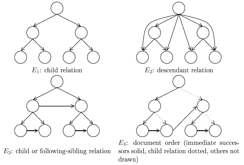
Figure 4:
Examples of different document graphs for the same document. E1 uses the
parent-child relation, E2 the ancestor-descendant relation (excluding
"self"), E3 the union of the parent-child and following-sibling
relations, and E4 a relation representing a pre-order traversal through
the document tree ("document order").
[Graphic entity document-graphs — PMS-FB-2005-11/ExML05/EML2005SCHA031802.png]
|
4 Node Similarity Relations, Nodeset Correspondence, and Retained Relations
In the following, we will introduce three additional kinds of relations. In order to not
confuse them, we give a brief overview over them here:
- a nodeset correspondence is a mapping
representing a solution; it describes where nodes of the first document are located in
the second document; the actual difference are obviously those nodes not contained in
the nodeset correspondence.
- the node similarity relation defines
which nodes are considered to be "similar" (e.g. those with the same label, or those
whose label has the same meaning); all nodeset correspondences are a subset of this
node similarity relation
- the retained relations (wrt. a nodeset
correspondence) are those relations between nodes in a single document
(e.g. parent-child) for which there exists a corresponding relation in the second
document
4.1 Nodeset Correspondence
A nodeset correspondence is an abstract representation of a "solution" to the
differencing problem, independent from the "edit script" generated as output.
It is a mapping from nodes of the (document graph of the) first document D=(V,E)
to nodes from the (document graph of the) second document D'=(V',E').
Informally, it describes where nodes of the first document are located in the
second document. Formally, it is a binary relation (or "one-to-one mapping") of
the form S={(v,v') | v ∈ V ∧ v' ∈ V'} with the additional restriction
that each v and each v' may occur at most once.
Therefore, we shall usually write S(v)=v' when we mean (v,v') ∈ S.
For a given pair of documents, there are many different nodeset
correspondences. Even the empty relation can be a nodeset correspondence, meaning
that the two documents have "nothing in common". In this case, the delta returned by
the algorithm would be to replace the first document by the second. Figure 5 illustrates different nodeset
correspondences for two example documents.
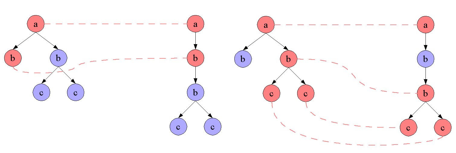
Figure 5: Nodeset Correspondences
Two different nodeset correspondences for the graphs induced by two XML
documents using label equality as node similarity relation; the correspondence on
the left simply relates the root nodes and the "b"-node of the left subtree with
the immediate "b"-node in the second document; the correspondence on the right
recognises the insertion of an additional "b"-node and is therefore of higher
"quality".
[Graphic entity nodeset-correspondances — PMS-FB-2005-11/ExML05/EML2005SCHA031803.png]
|
In principle, nodeset correspondences can be arbitrary mappings. We determine the
nodeset correspondence that is considered as "the solution" by using further quality
measures. These are characterised by the maximal nodeset
correspondence, by the node similarity
relation, and by a structure retainment
measure described in the following sections. The node similarity relation
and structure retainment measure can be influenced by the user to reflect his
specific needs. By appropriately choosing both, our approach also allows to model
some of the other algorithms described in the previous section.
4.2 Maximal Nodeset Correspondence
Although in principle all kinds of nodeset correspondences can be solutions, we are
usually only interested in those nodeset correspondences that determine a maximal set of nodes common to both documents. Formally, a
nodeset correspondence S1⊂~ is called maximal, if there exists no
nodeset correspondence S2 ⊆ ~ such that S1⊂
S2 and S1 ≠ S2 – i.e. there is no other
nodeset correspondence such that S1 is completely part of it. Note that
there still might exist several different maximal nodeset correspondences for two
XML documents, as illustrated in Figure 6.
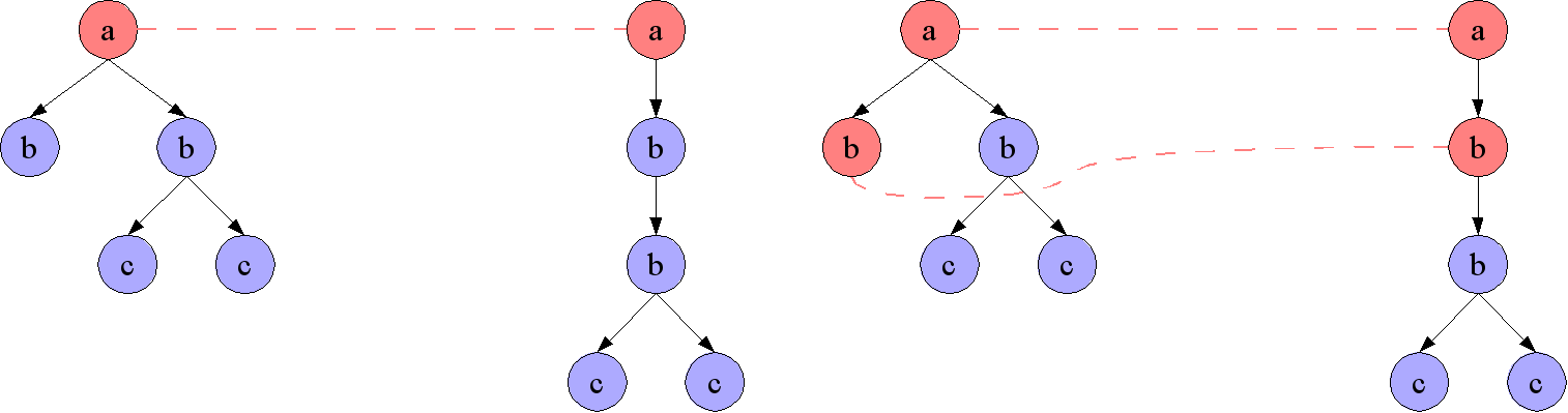
Figure 6: Maximal and Non-Maximal Nodeset Correspondences
The Figure on the right shows a maximal nodeset correspondence (from Figure 5), the Figure on the left a non-maximal
nodeset correspondence (subsumed by the nodeset correspondence on the right).
[Graphic entity nodeset-correspondance-maximal — PMS-FB-2005-11/ExML05/EML2005SCHA031804.png]
|
4.3 Node Similarity Relation
A nodeset correspondence mapping nodes from the first document to totally different
nodes in the second document is obviously undesirable. In this section, we therefore
describe so-called node similarity relations that
characterise the "acceptable" solutions and thus restrict the set of possible nodeset
correspondences. All (acceptable) nodeset correspondences between two documents are
required to be a subset of a node similarity relation chosen by the user.
The most straightforward node similarity relation simply considers two nodes as equal
when their labels are equal. Indeed, this is the similarity relation implemented in
most existing XML differencing applications. While this is satisfactory in many
cases, this approach is rather naive and easy to extend to cover also more complex
scenarios, e.g. considering two nodes equal if they are semantically equal (like the
"em" and "i" elements in XHTML), or if the two documents have similar schemas only
differing on certain element names. A more complex example would allow a label
s1 from the first document to match a label s2 in the second
document if s1 is a substring of s2. In principle, any kind of
binary relation between node labels describing what node labels are considered to be
equal is conceivable.
While this generalisation allows for some interesting use cases, they do not add much
complexity to the problem. For understanding the process here it is therefore
sufficient to simply assume that two nodes match if they have the same label.
We use the following notion of node similarity: a node v ∈ V from the first
document D=(V,E) is called similar
(denoted v ~ v') to a node v' ∈ V' from the second document D'=(V',E') if we
allow that v can be mapped to v' in a nodeset correspondence. Hence, the similarity
relation ~ is just the union of all acceptable nodeset correspondences, and each
one-to-one mapping that is a subset of ~ is a possible solution.
Formally, ~ is a relation ~⊆ V × V' where V are the nodes of the
document graph of the first document D=(V,E) and V' are the nodes of the document
graph of the second document.
Note that ~ may be an arbitrary relation between V and V' – including the empty set.
In that case, no node can have a match in the other document, and the differencing application always returns that
the documents have nothing in common. When the relation is a one-to-one mapping, there is only one solution.
Since there are so many different relations possible, the node similarity relation
can in most cases not be derived from the data or the schemas (to a certain amount,
relying on a dictionary or ontology can be an interesting solution, though). Instead,
the user of the differencing application needs to specify the similarity relation to
reflect his requirements and restrictions. We only allow solutions which are subsets
of the given relation. In most cases, defaulting to label equality will produce good
results.
Usually, one node will be similar to many nodes from the other document. There will
also often be nodes with no or only one node similar to them. Complexity of the task
is largely defined by this ratio: If we have two documents with n nodes each, and
every node in each document is similar to exactly one node in the other document,
then there is only one (maximal) solution. If every of these nodes is similar to
every node in the other document, then there are n! different (maximal) solutions
(e.g. compare matching two XML documents with nodes "a" to "z" each to comparing two
documents with 26 "a" nodes each).
4.4 Structure Retainment Measure
A further way of comparing different solutions is to measure the "quality" or
"importance" of the relations retained in a nodeset correspondence. The core
assumption of the approach presented here is that users can find better solutions by
choosing an appropriate structure retainment measure for their particular case.
A relation (e.g. parent-child) v → w ∈ E (v,w ∈ V) between two nodes
in a document D=(V,E) is considered "retained" by a nodeset correspondence S iff
S(v) = v', S(w) = w' and v' → w' ∈ E' is a relation in the other document
D'=(V',E'). That is, S maps the relation between nodes in the first document to a
corresponding relation between nodes in the second document.
Figure 7 illustrates this on two sample documents.
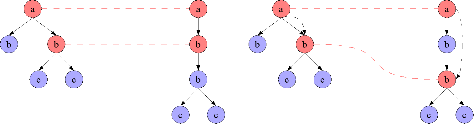
Figure 7: Retained Relations
The nodeset correspondence on the left retains the parent-child relation between
the node labeled "a" and the node labeled "b", whereas the nodeset correspondence
on the right doesn't. However, the nodeset correspondence on the right still
retains the ancestor-descendant relation (shown as a dashed arrow).
[Graphic entity retained-relation — PMS-FB-2005-11/ExML05/EML2005SCHA031805.png]
|
If we have measures ϕ1: V×V
→ R0+ and ϕ2:
V'×V'→R0+, and a combination rule
(e.g. ϕ(v,w,v',w')=ϕ1(v,w)+ϕ2(v',w')
or a similar multiplicative rule) we get a measure to compare solutions:
ψ(S) := ∑v,w∈V ∧ v→w∈E
∑v',w'∈V' ∧ v'→w'∈E' ∧ S(v)=v' ∧ S(w)=w'
ϕ(v,w,v',w')
In the remainder of the document we will assume the combination is done additively,
since this is the simplest case. Other combination rules can be approximated by using
the maximum of all possible combinations. Additive behaviour showed the intended
results, no experiments with other combination rules have been made so far.
5 Finding the Best Solution
Given the large number of possible nodeset correspondences (even when restricted to the
maximal nodeset correspondences), considering every single of them is
prohibitive. Luckily, efficient search algorithms considering only small fragments of
the search space have been available for a long time. For the purpose of our structure
based differencing, we use "Dijkstra's Algorithm" (for shortest-path search),
because it has the nice property to always determine the solution with the lowest cost,
albeit possibly with a slightly increased space and time complexity (depending on the
quality of the cost estimation function). For more efficient evaluation, extensions of
our algorithm could use A* search with an appropriate cost estimation function.
5.1 Dijkstra's Algorithm
Dijkstra's Algorithm is a graph algorithm solving
the shortest-path problem for a directed graph (and thus in particular for a search
tree) with nonnegative edge weights ("costs"). It is named after its inventor, Edsger
Dijkstra and described at numerous places (e.g. WikiPedia). This algorithm is often
taught in school, since it has numerous uses, is efficient and easy to understand.
Dijkstra's Algorithm takes as input a directed, weighted graph and an initial node
(called the "source"). The algorithm tries to determine a cost-optimal path from the
initial node to one of the goal nodes. In the following, we denote the cost of a
path in the search graph from the initial node to some node n (not necessarily a goal node) by c(n) and call c(.) the
cost function.
The algorithm (see Fig. 8) is straightforward: it
begins with the initial node and adds all its successors to a priority queue ordered
by the cost determined by the cost function c(.). It proceeds by selecting in each step the first node
of the priority queue (i.e. the one with the least cost) and adds all its successors
to the priority queue (which are thus rearranged according to the cost function). The
algorithm terminates when the selected node is a goal node.
Figure 8: Dijkstra's Algorithm
Dijkstra's Algorithm in a Python-like pseudo code notation
queue = []                   /* priority queue containing nodes */

initialNode.actual_cost = 0  /* initial node has no actual cost */

queue.insert(initialNode)

while not queue.isEmpty():
  candidate := queue.first()

  if isSolution(candidate):
     return candidate        /* best solution found; break loop */

  else:
     for nextNode in candidate.successors() do:

       queue.insert(nextNode)

     /* order queue ascending by path cost */
     queue.sortBy(lambda x,y: cmp(c(x),c(y)) )

return "no solution found"
|
5.2 States and State Transitions in the Search Graph
To avoid confusion between the different graphs and trees, we shall in the following
call the nodes of the search graph states, and
the goals solutions. Accordingly, edges in the
search graph are called state transitions.
Each state in the search graph represents a
nodeset correspondence. Additionally, each state stores information such as the
current position in the first document, the current costs and "credits" data used to
calculate costs, as explained later. The initial state represents the empty nodeset
correspondence (not mapping any nodes). The state is a solution if the
represented nodeset correspondence is maximal. Each state
transition adds an additional pair of nodes from the two documents to the
nodeset correspondence. For technical reasons, we also allow nodes from both
documents to be associated with a "null-node" (denoted ⊥) meaning that the node
has no corresponding partner in the other document. Intuitively, mapping a node to
⊥ thus means that the node is "skipped".
If we simply search the complete search space without making use of a cost function,
there are therefore O(nn+m) possible paths from the initial state to a
solution (i.e. maximal nodeset correspondence), where n is the number of nodes in the
first document and m is the number of nodes in the second document. Also, every path
in the search graph will be at most of length min(n,m). A simple optimisation is to
always add pairs in a fixed order given e.g. by enumerating the nodes in the first
document in "document order" (depth first left to right traversal).
5.3 Cost Function 1: Measuring the Number of Un-Retained Relations
Our first approach towards an appropriate cost function is straightforward: for each
state, we simply measure the number of relations not retained in the associated
(partial) nodeset correspondence. A relation a → b in one of the documents is not retained
by a state if it maps a and b to nodes a' and b' such there exists no corresponding
relation between a' and b'. This in particular holds if a, b, a', or b' are mapped to
the null-node ⊥. Note that a cost can only be evaluated for relations between
nodes that have already been processed by the algorithm (i.e. nodes for which the
nodeset correspondence provides a mapping).
Formally, the cost function is the sum over all weights (as given by the measure used
for structure retainment) of relations not
retained, i.e. for a state S. documents D=(V,E) and D'=(V',E') (V/V' vertices,
E/E' edges in the respective document graphs), and a "measure" ϕ:
Let S ⊆ V × V' be a nodeset correspondence ("state"), and let W ⊆ V and W'
⊆ V' be the nodes for which S already provides mappings. Also, let F = E|W
× W denote the restriction of E to only the nodes in W, and let
F' = E'|W' × W' denote the restriction of E' to only the nodes in W'.
The cost function c1 is defined (in Python pseudo-code) as
def c_1(State S):
  cost = 0

  /* check for retainment of all relations in F */
  for (a,b) in F:
    (a,a') in S
    (b,b') in S
    if not (a',b') in F':

      /* relation (a,b) is not retained in F' */

      cost = cost + weight(a,b)

  /* check for retainment of all relations in F' */
  for (a',b') in F'
    (a,a') in S
    (b,b') in S
    if not (a,b) in F:

      /* relation (a',b') is not retained in F */

      cost = cost + weight(a',b')

  /* return total cost */
  return cost
|
It is easy to see that this cost function is well-suited for our notion of
structure retainment - it describes exactly the amount of document structure
not retained. Indeed, for "solutions" this cost function fulfils the equation
retained structure =
structure in first document +
structure in second document -
structure lost (costs)
and by minimising the "structure lost" we can maximise the "retained structure".
Unfortunately, this cost function has a low selectivity especially at the beginning
of the search process, since we can only compute costs for relations where both nodes
have been mapped. If nodes are processed in an inauspicious sequence, this means we
have to expand half of the search graph before being able to compute any costs.
5.4 Cost Function 2: Credits for Unavoidable Droppings
Our second approach tries to increase the selectivity of the search algorithm by
taking into account that dropping certain relations is unavoidable, because the first
document contains a different number of relations between nodes with similar labels
than the other document. Consider for instance two documents where the first document
contains two a → b (for node labels "a" and "b", using label equality) relations
and the second document contains only one a → b relation; since every node is
associated with at most one other node (or the null-node), at least one of the
a → b relations of the first document has to be dropped.
Informally, we partition the nodes in each of the two documents in equivalence
classes according to label equality (other node similarities can be used, too)
in advance to the actual search, and count for each document and each pair of
equivalence classes the number of edges between nodes in those two classes.
Then we simply subtract for each pair of equivalence classes the number of edges
in the second document from the number of edges in the first document.
This gives us a so-called credit, where
a positive credit means that dropping edges contained in the first document is
unavoidable, and a negative credit means that dropping edges in the second document
is unavoidable. When we do the actual search, we associate a cost of zero when we
drop a relation as long as there is still "credit" for this relation. The rationale
for this is that every solution will have to drop at least as many relations as
indicated by the credit.
Figure 9: Credits for Cost Function 2
Consider the following two XML documents:
<a>             <a>
  <b>                <b>
    <c/>               <c/>
    <d/>               <c/>
  </b>                 <d/>
  <b>                </b>
    <e/>           </a>
  </b>
</a>
For both documents, we consider the equivalence classes a, b, c, d, and e. The following table summarises the numbers of
relations between these classes (only those relations with a count of more than 0
in one of the two documents are given):
         Document 1     Document 2      Credit
a → b    2              1                +1
b → c    1              2                -1
b → d    1              1                 0
b → e    1              0                +1
The credit figures state, for instance, that we are allowed to drop one a → b
relation of the first document at no cost, because the drop is unavoidable anyway.
|
As before, let S ⊆ V × V' be a nodeset correspondence ("state"), let W
⊆ V and W' ⊆ V' be the nodes for which S already provides mappings, let F =
E|W × W denote the restriction of E to only the nodes in W, and let
F' = E'|W' × W' denote the restriction of E' to only the nodes in
W'. In addition, let credits(a,b) be the credits value of the relations between nodes
labeled "a" and "b" as described above, determined in advance of the search
process. The cost function c2 is defined (in Python pseudo-code) as
def c_2(State S):
  cost = 0

  /* check for retainment of all relations in F */
  for (a,b) in F:
    (a,a') in S
    (b,b') in S
    if not (a',b') in F':
      if credits(a,b) < 1:
        /* no positive credit for a → b relations left */
        cost = cost + weight(a,b)
      else:
        /* enough credits left, no additional cost */
        /* relation (a,b) is not retained in F', deduce one credit */
        credits(a,b) = credits(a,b) - 1

  /* check for retainment of all relations in F' */
  for (a',b') in F'
    (a,a') in S
    (b,b') in S
    if not (a,b) in F:
      if credits(a,b) > 1:
        /* no negative credit for a → b relations left */
        cost = cost + weight(a',b')
      else:
        /* enough credits left, no additional cost */
        /* relation (a',b') is not retained in F, add one credit */
        credits(a,b) = credits(a,b) + 1

  /* return total cost */
  return cost
|
The restriction given by the node similarity already restricts the search
space, but also allows for a more "predictive" cost calculation. Steps that
only lose relations that we would lose in any case are "cheaper" with this
cost function. For example in a case, where one document is a true subtree
of the other document, no costs will be assigned by this cost function.
But this cost function still suffers to almost the same degree as the first
cost function from inauspicious processing sequence.
5.5 Cost Function 3: Incremental Calculation and Credit Updates
The third cost function adds two further improvements to the calculation: first,
instead of repeating the whole cost calculation process for every state anew, we
compute the costs incrementally by taking the costs of the previous state and
considering only the costs entailed by the mapping that is added to the nodeset
correspondence; second, instead of using a fixed, predetermined table of credits, we
allow for dynamic updates of the credit table in state transitions. Obviously, the
second improvement fits well with the first.
In terms of implementation, this means that we need to store for each state not only
the associated nodeset correspondence and current document position, but also the
current costs and the current credit table. In the initial state of the search graph,
the credit table is initialised with the fixed credit table of the second cost
function, and the current cost is initialised with 0. When transitioning from a state
S1 to a successor state S2, we add exactly one new mapping
(v,v') to the nodeset correspondence of S1, and examine the document
relations involving v and v'.
-
If a relation a → b is dropped and there is credit left, we simply update
the credit table and deduce (or add, in case the relation is in the second
document) one credit for a →
b, but keep the costs unmodified.
-
If a relation a → b is dropped and there is no credit left, we calculate the additional cost
resulting from dropping the relation and add it to the cost of
S1. Furthermore, dropping a relation without credit in one document
allows us to predict that dropping a corresponding a' → b' relation in the
other document becomes unavoidable, and we can add its costs immediately. To
account for this additional cost, we update the credit table by further
deducing/adding one credit (even beyond 0), thus permitting the now unavoidable
dropping of the relation at a later state with no costs (we already added the
associated costs). In a sense, we thus dynamically "create" new credit during
the traversal of the search graph. This refinement allows to predict costs very
early and thus increase the selectivity of the algorithm.
Let in the following S_1 ⊆ V × V' and S_2 ⊆ V × V' be nodeset
correspondences such that S_2 = S_1 ∪ { (v,v') }, i.e. S_2 contains exactly one
additional mapping (v,v') (the increment). Also, let E_I ⊆ E be all relations
involving v on either side (increment for E), and let E_I' ⊆ E' be all relations
involving v' on either side (increment for E'). Furthermore, for the states S_1 and
S_2, we denote with S_1.costs/S_2.costs and S_1.credits/S_2.credits the current cost
and current credits table of S_1/S_2. The cost function (or rather "state transition
function") c_3 is defined (in Python pseudo-code) as follows:
def c_3(State S_1, State S_2):
  /* continue calculation with previous values */
  S_2.costs   = S_1.costs
  S_2.credits = S_1.credits

  /* check for retainment of all relations involving v */
  for (a,b) in E_I:
    (a,a') in S_2
    (b,b') in S_2

    /* relation (a,b) is not retained in F', deduce one credit */
    S_2.credits(a,b) = S_2.credits(a,b) - 1

    if not (a',b') in E_I':
      if S_2.credits(a,b) < 0:
        /* no positive credit for a → b relations left;
           add costs for the  dropped relation and the
           predicted drop in the other document */
        S_2.costs = S_2.costs + weight(a,b) + weight(a',b')
      else:
        /* enough credits left, no additional cost */

  /* check for retainment of all relations involving v' */
  for (a',b') in E_I'
    (a,a') in S_2
    (b,b') in S_2

    /* relation (a',b') is not retained in F, add one credit */
    S_2.credits(a,b) = S_2.credits(a,b) + 1

    if not (a,b) in E_I:
      if S_2.credits(a,b) > 1:
        /* no negative credit for a → b relations left;
           add costs for the  dropped relation and the
           predicted drop in the other document */
        S_2.costs = S_2.costs + weight(a',b') + weight(a,b)
      else:
        /* enough credits left, no additional cost */

  /* return new state */
  return S_2
|
5.6 Cost Function 4: Processing Incompletely Mapped Relations
So far, the cost functions were only able to compute costs for relations for which
both nodes were part of the nodeset correspondence for at least one of the two
documents. Consequently, the nodeset correspondence needs to contain at least two
node mappings for the algorithm to compute any costs at all, still resulting in a
rather large branching of the search graph in early stages of the path search. Cost
Function 4 tries to improve this situation by predicting costs for future relation
drops in cases where only one of the nodes of a relation is already mapped.
For instance, if we transition to a new state by mapping a node a from the first
document to a node a' in the second document, we also process relations a →
b (for all partitions b) in the first and a'
→ b in the second document (a and b being the
equivalence classes of a and b wrt. node similarity). We can of course not yet know
precisely which of these relations we will be able to retain – but we can predict how
many of them will have to be given up at least by a rather simple calculation:
if there exist two a → b relations for the
node a to some node labeled b (not yet mapped by the nodeset correspondence), and
there exists only one a' → b' relation for
the node a' corresponding to a, at most one of the relations of a can be retained.
As before, let S_1 ⊆ V × V' and S_2 ⊆ V × V' be nodeset
correspondences such that S_2 = S_1 ∪ { (v,v') }, i.e. S_2 contains exactly one
additional mapping (v,v') (the increment). Also, let E_I ⊆ E be all relations
involving v on either side (increment for E), and let E_I' ⊆ E' be all relations
involving v' on either side (increment for E'). Furthermore, for the states S_1 and
S_2, we denote with S_1.costs/S_2.costs and S_1.credits/S_2.credits the current cost
and current credits table of S_1/S_2. The cost function (or rather "state transition
function") c_3 is defined (in Python pseudo-code) as follows:
def c_4(State S_1, State S_2):
  /* calculate costs by c_3 */
  S_2 = c_3(S_1, S_2)

  /* now process the additional relations */

  /* empty map used for counting relations involving v and v' */
  partition_sizes = { }

  /* count relations of a in E_I and update partition count
     (either a or b is v)                       */
  for (a,b) in E_I:
    /* update partition count */
    partition_sizes(a,b) = partition_sizes(a,b) - 1

  /* count relations of a' in E_I' and update partition count
     (either a' or b' is v', only the difference is relevant) */
  for (a',b') in F'
    /* update partition size */
    partition_sizes(a',b') = partition_sizes(a',b') + 1

  for (a,b) in partition_sizes.keys():
    /* the partition size value is 0, if there is an equal number of
       open relations. nonzero values mean a local imbalance */

    if partition_sizes(a,b) > 0:
      /* second document contains more relations, imbalance! */

      if S_2.credits(a,b) < partition_sizes(a,b):
        /* if we do not have sufficient credits, update costs */

        S_2.cost = S_2.cost + weight(a,b) *
                     (partition_sizes(a,b) - S_2.credits(a,b))

    if partition_sizes(a,b) < 0:
      /* first document contains more relations, imbalance! */
      if S_2.credits(a,b) > partition_sizes(a,b):
        /* if we do not have sufficient credits, update costs */

        S_2.cost = S_2.cost + weight(a,b) *
                     (S_2.credits(a,b) - partition_sizes(a,b))

    /* update credits, we added the expected costs above */
    S_2.credits(a,b) = S_2.credits(a,b) + partition_sizes(a,b)

  /* return new state */
  return S_2
|
6 Experimental Results
Visualising results of this approach is difficult. We would be happy to present
numerical results on how our algorithm compares to others, but to compute the number of
retained relations we would need a rather complex program to reinterpret the edit
scripts produced by other algorithms (which usually only have an edit-script
output). Instead of numerical results about retained relations, we thus simply show the
different edit scripts produced by Logilab's xmldiff and our prototype.
Note that our prototype currently only supports the most advanced cost function (c_4),
so we currently cannot compare the different cost functions on real examples. An
extension of the prototype is currently being worked on.
Most examples, especially with "real world documents", would require big XML documents
to be included in this document, bloating it unnecessarily. Also XML edit scripts are
often again XML documents and rather hard to read without the help of applications or
special formatting. Therefore, we decided to only use small, artificial samples, and
describe the difference intuitively without giving the actual output of the different
algorithms. Interested readers can find a more extensive collection of examples in
[Schubert, 2005].
6.1 First example – Quality of result
In this example we want to illustrate that the results produced by our algorithm are
sensible, and are more likely to reflect the actual change than other XML
differencing tools. We show two documents and "natural language" transcription of
the edit script produced by our prototype and Logilab xmldiff. Logilab xmldiff was
chosen because it is included in the Debian GNU/Linux distribution and actually
intended for end-users. Installation is as easy as one click in the package manager.
It should be said that it (now) uses an approximative algorithm for speed reasons,
not always producing the optimal result. In the process of testing our application we
also provided test cases and feedback to the Logilab developers. We did not compare
speed or memory usage of Logilab xmldiff and our prototype, Logilab xmldiff likely is
better in this respect.
Our prototype application can be downloaded from
http://ssddiff.alioth.debian.org/. It requires only libxml and C++. It has so far
only been tested on Linux, but should work in other environments as well. There is no
graphical user interface.
Figure 10: Example documents to be compared
These are two example documents to be compared by our prototype application and
Logilab xmldiff. The difference obviously is that the "b" tag has been moved to a
different "node". In a real-life example, this could for example be a "em"
emphasis tag in HTML being moved to a different row of a table.
  <?xml version="1.0"?>            <?xml version="1.0"?>
  <root>                           <root>
    <sub>                            <sub>
      <node>0</node>                   <node>0</node>
      <node><b>1</b></node>            <node>1</node>
      <node>2</node>                   <node>2</node>
      <node>3</node>                   <node>3</node>
    </sub>                           </sub>
    <sub2>                           <sub2>
      <node>0</node>                   <node>0</node>
      <node>2</node>                   <node><b>2</b></node>
      <node>3</node>                   <node>3</node>
    </sub2>                          </sub2>
    <other/>                         <other/>
  </root>                          </root>
|
For running the prototype with the example documents given in Figure 10, we used child and "grandchild" relations each with a
weight of 1. This setting has shown to be a reasonable default for many cases. A
lower weight for "grandchild" relations would make sense, but is currently not
supported by our prototype.
The edit script output (our prototype can output XUpdate edit scripts as well as a
custom "merge" format and a format where nodes are marked with integer IDs to output
the final mapping) transcribed into natural language for readability is as follows:
- store and remove the contents of the "b" element
- store and remove the (now empty) "b" element
- reinsert the contents removed in step 1 at the place of "b"
- store and remove the contents of the destination "node"
- insert the "b" tag removed in step 2 at destination "node"
- insert the old contents of the destination node into the "b" tag
This edit script is pretty much what a human would write, when given
only this limited set of operations.
The Logilab xmldiff output transcribed into natural language is:
- rename the "b" element to "node"
- move the just renamed "node" element one level up
- remove the "node" the (now renamed) "b" was in
- rename the other modified "node" element to "b"
- add a new element "node" below it
- move the "b" element into the newly generated element
In our conviction, these changes are counterintuitive: instead of
removing the "b" tags, they are renamed from and to "node" tags, and
a "node" tags is removed and added instead. This probably is a
consequence of the algorithm used, which appears to work by bottom-up
extending identical subtrees.
6.2 Second Example – User-Supplied Parameters
With the second example, we want to illustrate that there isn't the "perfect" diff,
but that the user may prefer one or another, depending on his preferences, the use
and the document type. For this purpose, we again use two example documents, modeled
according to an imaginary "document" format. We obtain two different results from
these documents, and present a rationale for each of them. Both results have been
obtained by using different parameters in our prototype.
Figure 11: First document for second example
This XML file reflects a typical structure of a word processing document, without
much content to keep the example small.
<?xml version="1.0"?>
<root>
  <part>
    <title>Title text</title>
    <subtitle>First subtitle</subtitle>
    <content>
      <text>
        <par>First text content, first paragraph</par>
        <par>First text content, second paragraph</par>
      </text>
    </content>
  </part>
  <part>
    <title>Second title</title>
    <subtitle>Second subtitle</subtitle>
    <content>
      <text>
        <par>Second text content, first paragraph</par>
        <par>Second text content, second paragraph</par>
      </text>
    </content>
  </part>
</root>
|
Figure 12: Second document for second example
The difference to the first document is merely in the text parts of the "par"
nodes (which have been swapped). In a real-world case, the author might for
example have rearranged paragraphs.
<?xml version="1.0"?>
<root>
  <part>
    <title>Title text</title>
    <subtitle>First subtitle</subtitle>
    <content>
      <text>
        <par>Second text content, first paragraph</par>
        <par>Second text content, second paragraph</par>
      </text>
    </content>
  </part>
  <part>
    <title>Second title</title>
    <subtitle>Second subtitle</subtitle>
    <content>
      <text>
        <par>First text content, first paragraph</par>
        <par>First text content, second paragraph</par>
      </text>
    </content>
  </part>
</root>
|
The output format used in the following is the "merged" output format of the
prototype implementation. It uses attributes and additional nodes in the
"merged-diff" namespace (using the "di:" prefix here) to mark changes in the
document. This is usually easier to read than XUpdate statements, and the files are
often still valid documents. The output has been slightly reformatted by using
additional whitespace for printing.
The first result shown in Figure 13 was obtained by
using the XPath expression "./* | ./*/*" as relations to be retained. This expression
relates nodes with children and grand children each with a weight of 1. This is the
default setting of the prototype, producing useful results in many cases. The result
can be interpreted as removing the text contents and inserting them at their new
location. This result is probably what most users will have expected.
Figure 13: First result for second example
This is the "merged" result produced by our prototype when run with default
options. The "di" ("merged-diff") namespace is an experimental format to mark
changes. Unchanged parts are not marked.
<?xml version="1.0"?>
<root xmlns:di="merged-diff">
  <part>
    <title>Title text</title>
    <subtitle>First subtitle</subtitle>
    <content>
      <text>
        <par>
          <di:removed-text di:following="moved-here">First text content, first paragraph</di:removed-text>
          Second text content, first paragraph</par>
        <par>
          <di:removed-text di:following="moved-here">First text content, second paragraph</di:removed-text>
          Second text content, second paragraph</par>
      </text>
    </content>
  </part>
  <part>
    <title>Second title</title>
    <subtitle>Second subtitle</subtitle>
    <content>
      <text>
        <par><di:removed-text di:following="moved-here">Second text content, first paragraph</di:removed-text>
          First text content, first paragraph</par>
        <par><di:removed-text di:following="moved-here">Second text content, second paragraph</di:removed-text>
          First text content, second paragraph</par>
      </text>
    </content>
  </part>
</root>
|
Our merge format uses "<di:removed-text>" to wrap text content that is removed
from the first document, and adds a 'di:following="moved-here"' attribute to mark
inserted text (since text cannot have attributes, we have to mark it on the preceding
node in document order. This merge format is of experimental nature and has not been
formalised (attribute handling is problematic).
But this result is not always what the user wants to obtain. In many document types,
text contents should always have a surrounding tag, which specifies the meaning of
the actual text (in this case, stating that the text is a paragraph, not a title).
By a slight tweak to our prototype – by using the XPath expression
"self::*[not(name()='text')]/node()" to define the relevant relation – we can
obtain a different result. This expression specifies "all child relations, except
those from text to par nodes". If our prototype had support for different weights,
we could have assigned a low weight such as 0.1 to these relations to obtain the same
effect for these documents.
Arguably, many users will find the result shown in Figure 14 easier to read than the first result. Instead of just
moving the text contents, now whole "paragraphs" are moved. Our "merged" output
format should be self-explanatory here – nodes with the "moved-away" attribute
were at this position only in the first document, nodes with "moved-here" only in the
second.
Figure 14: Second result for second example
A different result obtained from the same input documents, by
passing a different parameter to the prototype application.
<?xml version="1.0"?>
<root xmlns:di="merged-diff">
  <part>
    <title>Title text</title>
    <subtitle>First subtitle</subtitle>
    <content>
      <text>
        <par di:n="moved-away">First text content, first paragraph</par>
        <par di:n="moved-away">First text content, second paragraph</par>
        <par di:n="moved-here">Second text content, first paragraph</par>
        <par di:n="moved-here">Second text content, second paragraph</par>
      </text>
    </content>
  </part>
  <part>
    <title>Second title</title>
    <subtitle>Second subtitle</subtitle>
    <content>
      <text>
        <par di:n="moved-away">Second text content, first paragraph</par>
        <par di:n="moved-away">Second text content, second paragraph</par>
        <par di:n="moved-here">First text content, first paragraph</par>
        <par di:n="moved-here">First text content, second paragraph</par>
      </text>
    </content>
  </part>
</root>
|
7 Perspectives and Conclusion
There are different possibilities to increase the speed of the algorithm
or enhance its usage possibilities:
7.1 Optimised Traversal
Both the speed of the algorithm and the memory usage depend on the
order the nodes are processed. Finding the optimal sequence needs
further investigation of good and bad cases for the algorithm. Using
the document order, as currently employed in the implementation, is
likely to not be optimal.
Strategies might include sorting the nodes by similarity class cardinality,
or by the number of relations the node participates in.
The general approach should be to try to keep the number of low-cost
choices low at the beginning, to avoid a too broad search.
7.2 Reducing the Number of Equivalence Classes
The memory usage is up to quadratic in the number of equivalence classes.
This can be reduced by merging equivalence classes. Depending on the
document, such merges may not make a difference to the quality of
the cost estimation function.
7.3 Search Tree Pruning
To reduce memory usage, "dead ends" of the search tree should be pruned from the
tree. For example, if there is a partial solution already retaining 30 of 50 possible
relations, any partial solution with a cost of 20 (that would never be considered
again) can be dropped. This frees memory for storing new open ends of the search
tree.
7.4 Divide and Conquer Strategies
Currently, the algorithm searches for a path through the whole document. To find a
possibly better path it might be necessary to step back much and redo the same search
for the next nodes again. A typical case is when processing the next subtree of a
document – finding the optimal match for one subtree is already a complex
search task; having to step back from the second subtree to try an alternative in the
first subtree is "expensive", usually meaning to have to redo the second subtree from
scratch (when processing in document order, processing in classes or any other order
has similar troubles).
The alternative is to process similarity classes independently (or subtrees, but
similarity classes are easier to separate independently on the used relation), then
use a second level search, trying to combine the previous results. Basically the same
algorithm can be used, just that the steps made are not additions of single node
correspondences, but node set correspondences covering a whole class as returned by
earlier searches. When using this approach, the algorithm must not stop after having
found the first complete solution, rather looking at less optimal solutions for each
class might be required to get the best global result.
7.5 Approximative Solutions
A major drawback of the presented algorithm is the amount of memory needed, and the
expensive lookups whether a node has already been matched earlier.
When not caring about finding the optimal solution but only an approximation, a
possible approach would be to assume in each step that no nodes from a different
class have yet been fixed (i.e., only check which "similar" nodes are unmatched to
only return valid mappings, but not calculating the real costs but just using the
credit information).
This is similar to the previous "divide and conquer" approach, basically taking the
best result in each class and combining them to form the final solution without
looking at combinations with secondary results in the classes, but eventually
applying local optimisations techniques.
This approach can further be optimised for trees and DAGs by using index tables.
7.6 Solution Simplification
Currently, the algorithm will even match two nodes if no relation is retained at all,
as long as there is no better choice. There might be cases where single relations are
kept, such that the total number is maximal, still the solution is
counterintuitive. Such cases can probably not be detected automatically, but the user
might want to force the program to behave differently. For example, extra costs might
be assigned to nodes that keep none of their relations or only a small number or
small percentage of their relations. This can be used to prevent "stray matches".
7.7 Using DTD Information and DTD Learning
DTD ("Document Type Definition", language for describing the
format of an XML document) information could be used to optimise the
search process. For example to divide nodes with the same label into
different classes when they occur in different contexts (that have
a different meaning).
Also, automatic learning of DTD descriptions when given a set of example documents is
an interesting possible application.
7.8 Database Applications
Databases need a way to easily narrow down candidates for matching. X-Trees and
similar high-dimensional data structures could be used to store the number of
relations a node participates in (or a subtree contains) to easily narrow down the
amount of data to search in.
On the data indexing side, the path search cost function used here makes use of a
value to estimate costs that provides an ordering between elements that could show
useful in databases to partition the data space. On the query side, comparing a small
"query" document with a big "database" document is a typical usage for a query,
except that in most query cases you do not want to allow fuzzy matches. By using
infinite costs for relations lost in the "query" document, but normal costs for the
database document this can be solved.
Acknowledgments
This research has been funded by the European Commission and by the Swiss Federal
Office for Education and Science within the 6th Framework Programme project REWERSE
number 506779 (cf.
http://rewerse.net).
Bibliography
[Schubert, 2005]
Erich Schubert. Structure Preserving Difference Search in Semistructured
Data. Projektarbeit/Project Thesis, University of
Munich. Supervisors: François Bry and Sebastian Schaffert. 2005.
[Bry and Schaffert, 2002] François Bry and Sebastian Schaffert. Towards a
Declarative Query and Transformation Language for XML and Semistructured Data:
Simulation Unification. In Proceedings of the International
Conference on Logic Programming (ICLP), Copenhagen, Denmark, July
2002. Springer-Verlag, LNCS 2401.
[Schaffert, 2004]
Sebastian Schaffert. Xcerpt: A Rule-Based Query and Transformation Language for
the Web. PhD Thesis, University of Munich.
2004.
[Cobéna et. al., 2002a]
Grégory Cobéna, Serge Abiteboul, and Amelie Marian. Detecting Changes in XML
Documents. In International Conference on Data Engineering
(ICDE'02), San Jose, California, 2002.
[Chawathe et. al., 1996]
S. Chawathe, A. Rajarman, H. Garcia-Molina, and J. Widom. Change Detection in
Hierarchically Structured Information. In SIGMOD
25(2), 1996, pages 493-504.
[La Fontaine, 2002]
Robin La Fontaine. A Delta Format for XML: Identifying Changes in XML Files and
Representing the Changes in XML. In Proceedings of XML
Europe, Berlin, Germany, May 2001.
[Wang et. al., 2003]
Y. Wang, D. DeWitt, and J. Cai. X-Diff: A fast change detection algorithm for XML
documents. In International Conference on Data Engineering
(ICDE'03), Bangalore, India, 2003.
[Chawathe, 1999]
Chawathe, S. Comparing Hierarchical Data in External Memory. In International Conference on Very Large Databases (VLDB'99),
Edinburgh, Scotland, 1999
[XMLDiff]
Logilab XMLDiff. Project Website http://www.logilab.org/projects/xmldiff/ .
[IBM XML Diff and Merge]
IBM XML Diff and Merge Tools. Project Website
http://www.alphaworks.ibm.com/tech/xmldiffmerge .
[Cobéna et.al., 2002b]
Grégory Cobéna, Talel Abdessalem, and Yassine Hinnach. A comparative study for XML
change detection. In Research Report, INRIA Rocquencourt,
France, 2002.
[GNU Diffutils]
http://www.gnu.org/software/diffutils/diffutils.html
[XUpdate]
XML:DB Initiative: XUpdate - XML Update Language. http://xmldb-org.sourceforge.net/xupdate/